|
Quick reference:
Import the data. To calculate non-parametric reference intervals, select first Data Options. In the options window, choose Direct
calculation method, define the method for removing outliers (if any), define reference
limits (default 2.5% and 97.5%) and their confidence interval (either 90%, 95% or 99%,
default 90%). Select OK and Data Calculate. To print the output by your
printer, select File Print.
This procedure can be used for displaying the reference distribution and for
calculating non-parametric reference limits, median or any other percentiles of the
distribution. The frequency distribution is automatically formed from the source data
during the data import.
Output consists of two windows. The numerical frequency distribution is shown in the
left hand data window, in the right hand window the frequency distribution is shown as a
graph. The sizes of the windows can be adjusted by mouse by dragging at the borders. The
column widths in the data window can similarly be adjusted by the mouse by dragging at the
column borders on the title row. In the graphical frequency distribution, the x-value
corresponding to the cursor position is shown together with the corresponding percentile.
The values for the cursor position are updated each time the cursor is moved. By mouse
click, the defined confidence intervals (either 90%, 95% or 99%) for any percentile are
calculated and can be seen in a separate Current point window. For the calculation methods
that GraphROC uses, see Kairisto & Poola (1995).
The frequency distributions of clinical laboratory data are often difficult to display,
because the bin width may be quite small, the number of observations in the data set
limited and the total dispersion of results high. For the graphical presentation of such
data, it may be necessary to enlarge the bin width and exclude outliers for more
illustrative presentation (Kairisto, 1995). In this program, the regrouping of data with
new bin width can optionally be done either by using the statistically optimized or any
manually entered bin width. Outliers can be identified visually from the graph or the
Dixon's or the iterative � 4 SD principle can be used in outlier detection. The bin
widths and outlier removal method can be defined in the Data Options window. For
the mathematical formulas used by the program, see Kairisto & Poola (1995).
Both the original distribution and the regrouped distribution can be shown in the same
graph. Optionally, either of these distributions can alone be chosen for the graphical
presentation. The reference limits at selected percentile values can be chosen to be shown
in the graph as vertical lines together with the corresponding confidence limits as dotted
lines. For display of the histograms, either line or bar histogram can be selected. All
the display options mentioned above can be defined in the Graph Options window.
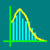
Figure 1. Graphical
output of reference distribution for serum lactate dehydrogenase (U/l) in 254 healthy
subjects. After calculation, defined reference limits with the corresponding confidence
limits are shown as vertical lines.
Figure 2. The same
distribution as above after optimization of the bin width for illustrative display. The
Current point window including data of the current percentile and its confidence limits
becomes visible by mouse click.
The graph can be printed together with the following numerical information: Original
reference distribution: number of observations, class width, mean, standard deviation,
lowest and highest value, (reference limits with corresponding confidence limits as
defined in the data options)
Regrouped reference distribution: number of outliers removed, used outlier removal
method, mean, standard deviation, class width, frequency of the mode class, lower limit of
lowest class, upper limit of highest class.
The printing is done by the Print File command. Before printing the program asks
for a title for the printed output. The title will be printed above the graph. Previewing
is also possible by the Print Preview command.
Any selected data in the left-sided data window can be exported via Windows clipboard to
other software running under Microsoft Windows by using the Edit Copy data command.
Also the graph from the right-sided window can be exported via clipboard by using the Edit
Copy graph command.
Quick reference
Import the data. The source data for the calculation of reference changes must consist of
delta-values (differences of two consecutive test results, the second result minus the
first result). To calculate the non-parametric reference change limits, select first Data Options. In the options window, choose direct calculation
method, define the method for removing outliers (if any), define the desired percentiles
for reference change limits (defaults 2.5% and 97.5%) and their confidence interval
(either 90%, 95% or 99%, default 90%). Select OK and Data Calculate. To
print the output by your printer, select File Print.
The direct non-parametric calculations are selected from calculation options window.
Source data for this procedure consists of differences of two consecutive laboratory tests
within the same patient. To obtain this difference, the value of the first test result
should be subtracted from the second result. Such source data files can be created by any
database or worksheet program. The difference can be either negative or positive. If the
value is negative, it should have the preceding minus sign, otherwise the value is
considered positive. The frequency distribution is automatically formed during the data
import. Output consists of two windows. The numerical frequency distribution is shown in
the left hand window, and in the right hand window the frequency distribution is shown as
a graph.
Handling of data and graph follow closely the procedures described above for reference
distribution. Several investigators have used this method for the calculation of reference
changes (Albert & Harris 1987; Shahangian et al. 1989; Kairisto et al. 1995).
Calculation of percentiles and their confidence limits, removal of outliers and
calculation of optimal bin widths are all done exactly in the same way as for ordinary
reference distributions.
Both the original reference change distribution and the regrouped reference change
distribution can be shown in the same graph. Optionally, either of these distributions can
alone be chosen for the graphical presentation. The reference change limits at selected
percentile values can be chosen to be shown in the graph as vertical lines. The confidence
intervals for reference change limits are shown as dotted vertical lines. This graph can
be printed together with the following numerical information:
Original reference change distribution: number of observations, class width, mean,
standard deviation, lowest and highest value, (reference limits with corresponding
confidence limits as defined in the data options)
Regrouped reference distribution: number of outliers removed, used outlier removal method,
mean, standard deviation, class width, frequency of the mode class, lower limit of lowest
class, upper limit of highest class.
The printing is done by the Print File command. Before printing, the program
prompts for a title of the printed output. The title will be printed above the graph.
Previewing is possible by the Print Preview command.
Any selected data in the left-sided data window can be exported via Windows clipboard to
other software running under Microsoft Windows by using the Edit Copy data command.
Also the graph from the right-sided window can be exported via clipboard by using the Edit
Copy graph command.
A: Indirect estimation of "health" related limits from
unselected or partially selected laboratory data distributions
Quick reference
To calculate indirect "health" related limits from routine laboratory data,
estimate first if the available source data meets the criteria listed below. If the answer
is yes, proceed as follows: Import the data. Select Data Options.
In the options window, choose Indirect and Ordinary limits, check that the method for
removing outliers is the �4 SD method, define the desired percentiles for the
limits (default 2.5% and 97.5%). Select Data Calculate. To print the output by your
printer select File Print.
In this procedure, the health related limits are roughly estimated from data obtained
from routine laboratory databases.
NOTE!
The indirect method does not follow the IFCC recommendations for the
production of reference limits, because in this, like in other indirect methods, reference
subjects are not individually selected. Therefore, we do not call the derived limits
reference limits. The method is not appropriate and should not be used if the following
prerequisites are not met for the analyte considered:
1. The health-related subdistribution must form a major part of the total distribution.
- This statement should be true for most "screening like" laboratory tests, but
for more specific tests the target population usually contains too many illness related
values for the method to be useful. Each patient should be included only once. This
exclusion of repeat tests within same individuals often removes many illness related
values. Hospital discharge diagnosis register can be used for estimating the prevalence of
the illnesses with effect on the considered laboratory test, and diagnosis-selection for
at least partial removal of the illness-related values before applying this method.
2. The total distribution must be unimodal, but can be skewed to either direction.
- This kind of distributions are typical of the most laboratory analytes. Bimodal
distributions can usually be divided into unimodal distributions by forming different
subdistributions, for example, for different sexes or for some other known classification
factor.
3. The values of the health-related subdistribution should be concentrated near the
mode of the total distribution, and the values in the tails of the total distribution
should predominantly be sickness-related.
- This, of course, is true if the laboratory test considered has a good clinical
sensitivity and specificity for the illness considered
4. The modes of the total distribution and the health-related subdistribution are the
same or quite close to each other and the health-related distribution can satisfactorily
be approximated with two halves of Gaussian distributions
- According to our empirical results, this is true for many distributions of clinical
chemistry laboratory data
The method was developed by utilizing some of the principles first described by Pryce
(Pryce, 1960) and Hoffmann (Hoffmann et al., 1964). The main modifications are the
splitting of the distribution into two unequal parts, and forcing the mode (rather than
the mean) of the health-related distribution to be the same as the mode in the original
distribution (N�nt�, Kairisto & Kouri, 1992). For a detailed description of the
mathematical methods, see Kairisto & Poola (1995). Note that the indirect method that
GraphROC uses is different from the earlier described indirect methods based on
distribution fitting (Gindler 1970; Naus et al. 1980; Baadenhuijsen & Smit 1985;
Oosterhuis et al. 1990).
For creating the underlying, supposedly health-related, distribution you first have to
define the calculation options in Data Options and perform
the calculations by Data Calculate. The calculation method should be Indirect and
for Ordinary limits. The preferrable outlier removal method is the iterative 4*SD method
and the Regrouping method should be the Optimal. The percentiles of the calculated limits
can be defined in Data Options.
The definitions made in Data Options will take effect
after calculation by selecting Data Calculate or alternatively after pressing Ctrl
and A buttons simultaneously.
The options for the graphical output can be defined in Graph Options.
All three distributions of the indirect method can be chosen for
simultaneous graphical display. These three distributions are:
1. Original distribution (original bin width)
2. Regrouped distribution (original distribution with optimized bin
width)
3. Underlying distribution (underlying, supposedly
"health" related distribution). This distribution consists of two split Gaussian
distributions, which have the same mode and frequency of the mode, but standard deviations
for each side can be different.
Underlying distribution is always shown as a line histogram, but for the original
and regrouped distributions, either bar or line histogram presentation can be chosen.
Maximum of four different values can be chosen to be updated for cursor position. The
defaults are that figures in the upper right corner of the graph tell the X-value (x scale value) and the corresponding percentile in the original
distribution (percentile in or. distr.), but also the Y-value (frequency, y scale value)
and the percentile in the underlying distribution (percentile in und. distr.) can be
selected. All four values will update if the cursor is moved
by the mouse.
The graphical output can be printed together with the following
numerical information:
Original reference distribution: number of observations,
class width, mean, standard deviation, lowest and highest value
Regrouped reference distribution: number of outliers removed,
used outlier removal method, mean, standard deviation, class width, frequency of the mode
class, lower limit of lowest class, upper limit of highest class.
Underlying distribution: mode, SD for left side, SD for right
side
Suggested health-related interval: lower limit and the
corresponding percentile in the underlying distribution, upper limit and the corresponding
percentile in the underlying distribution
Only those distributions, which have been selected for graphical
output in Graph Options, will be printed. The printing is done by the Print File
command. Before printing the program asks for a title for the printed output. The title
will be printed above the graph. Previewing is possible by the Print Preview
command. Any selected data in the left-sided data window can be exported via Windows
clipboard to other software running under Microsoft Windows by using the Edit Copy data
command. Also the graph from the right-sided window can be exported via clipboard by using
the Edit Copy graph command.
B: Indirect estimation of "health" related change limits from
unselected or partially selected laboratory data distributions
Quick reference
To calculate indirect "health" related change limits from routine laboratory
data, estimate first if the available source data meets the criteria listed below. If the
answer is yes proceed as follows: Import the data. The source data for the calculation of
reference changes must consist of delta-values (differences of two consecutive test
results, the second result minus the first result). Select Data Options. In the
Options window, choose Indirect and check that the method for removing outliers is the �4
SD method, define the desired percentiles for the change limits (default 2.5% and 97.5%).
Select Data Calculate. To print the output, select File Print.
In this procedure, the "health" related change limits are estimated from data
obtained from routine hospital databases. The source data should consist of delta values
(differences between two consecutive laboratory results, the second result minus the first
result). Note that this method differs from the direct calculation of reference change
limits in the sense that reference subjects are not individually selected. Instead, the
"health" related change limits are produced from routine data assuming that most
of the change values in source data are health related. The method has been recently
published by us (Kairisto et al. 1993).
NOTE!
The indirect method for reference changes should not be used if
the following assumptions of source data can not be considered correct
1. The health-related change data -subdistribution must form a major part of the total
change data distribution.
- This statement should be true for most "screening like" laboratory tests, but
for more specific tests the target population usually contains too many illness related
values for the method to be useful. Only one change value should be included from each
individual. Hospital discharge diagnosis register can be used for estimating the
prevalence of the illnesses which have effect on the laboratory test considered and
diagnosis-selection for at least partial removal of the illness-related change values
before applying this method.
2. The change values of the health-related subdistribution should be concentrated near
the mode of the total change data distribution (usually near zero), and the values in the
tails of the total distribution should predominantly be sickness-related.
- This, of course, is true if changes in the laboratory test considered have a good
clinical sensitivity and specificity for the illness considered
3. The modes of the total distribution and the health-related subdistribution are the
same or quite close to each other.
- Usually the modes of both the total and health-related change data distributions are
close to zero, but sometimes similar changes in preanalytical factors (for example, first
sample collected without preanalytical standardization at Emergency department and second
sample collected under more standardized conditions at Hospital ward) may affect the modes
of both distributions to deviate similarly from zero. The indirect method can be applied,
provided that the deviation can be estimated to be similar for all subjects.
4. The health-related subdistribution of changes can satisfactorily be approximated by
a Gaussian distribution.
- The distribution of changes tends to be a Gaussian distribution, independent from the
shape of the source distributions, provided that the changes represent random variation
and that the within-subject variances are homogeneous. Reference changes in general are
not very useful for analytes, which show heterogeneity in within-subject variances.
Within-subject time series analysis should be used for the analysis of serial results in
such cases (Albert & Harris 1987, Fraser & Harris 1989).
The method is based on fitting a Gaussian distribution to the central parts of the
distribution of all change values. The parameters for the Gaussian distribution are
obtained from frequency classes near the mode class so that the tails of the original
distribution have no effect on the Gaussian distribution (Kairisto et al. 1993). For a
detailed description of the mathematical methods, see Kairisto & Poola (1995).
For creating the underlying, supposedly health-related, change distribution you first
have to define the calculation options in Data Options and
perform the calculations by Data Calculate. The calculation method should be
Indirect and for Change limits. The preferrable outlier removal method is the iterative �4SD method and the Regrouping method should be the Optimal. The
percentiles of the calculated limits can be defined in the Data Options window.
Note that in the indirect method, the percentiles here refer to the underlying, supposedly
health-related, change distribution. In the indirect method, there is at present no system
available for the calculation of confidence intervals. We stress that the reliability of
the method is strongly dependent on how well the conditions numbered above are met.
The definitions made in Data Options will take effect first after calculation by
selecting Data Calculate or alternatively after pressing Ctrl and A buttons
simultaneously. The options for the graphical output can be defined in Graph Options.
All three change distributions of the indirect method can be
chosen for simultaneous graphical display. These three distributions are:
1. Original change distribution (original bin width)
2. Regrouped change distribution (original distribution with
optimized bin width)
3. Underlying change distribution (underlying, supposedly
"health" related change distribution). This distribution is a Gaussian
distribution, which has the same mode as the regrouped change distribution.
Underlying change distribution is always shown as a line
histogram, but for the original and regrouped distributions, either bar or line histogram
presentation can be chosen. Maximum of four different values can be chosen to be updated
for cursor position. The defaults are that figures in the upper right corner of the graph
tell the X-value (x scale value, the change value) and the corresponding percentile in the
original distribution of change data (percentile in or. distr.). However, also the Y-value
(frequency, y scale value) and the percentile in the underlying distribution of supposedly
"health" related changes (percentile in und. distr.) can be selected for
display. All four values will update if the cursor is moved by the mouse.
The graphical output can be printed together with the following
numerical information:
Original reference change distribution: number of
observations, class width, mean, standard deviation, lowest and highest value
Regrouped reference change distribution: number of outliers
removed, used outlier removal method, mean, standard deviation, class width, frequency of
the mode class, lower limit of lowest class, upper limit of highest class.
Underlying change distribution: mode, SD
Suggested health-related change interval: lower limit and the corresponding
percentile in the underlying change distribution, upper limit and the corresponding
percentile in the underlying change distribution.
Only those distributions, which have been selected for graphical
output in Graph Options, will be printed. The printing is done by the Print File
command. Before printing, the program asks for a title for the printed output. The title
will be printed above the graph. Previewing is possible by the Print Preview
command.
Any selected data in the left-sided data window can be exported
via Windows clipboard to other software running under Microsoft Windows by using the Edit
Copy data command. Also the graph from the right-sided window can be exported via
clipboard by using the Edit Copy graph command.
|